Quickstart

First ensure you have installed Python 3.5 (or greater), sparti and other common dependence packages. After installation you can start using Sparti:

import sparti

Sparti is easy to use. As long as you have specified the data, label, parameter and the task category, you can make it run and get the results!

Take BSPF (which is the Binary Space Partitioning Forest) as an example. First, you have the data (e.g. we are using the Friedman test data):

dimNum = 5
dataNum = 10000
xdata, ydata = sparti.BSPF.Friedman_function_gen(dimNum, dataNum)

The above would create the feature data (xdata) and label data (ydata).

For likelihood-free models we typically need to define a simulator and summary statistics for the data. As an example, lets define the simulator as 30 draws from a Gaussian distribution with a given mean and standard deviation. Let’s use mean and variance as our summaries:

Let’s now assume we have some observed data y0 (here we just create some with the simulator):

[[ 3.7990926   1.49411834  0.90999905  2.46088006 -0.10696721  0.80490023
   0.7413415  -5.07258261  0.89397268  3.55462229  0.45888389 -3.31930036
  -0.55378741  3.00865492  1.59394854 -3.37065996  5.03883749 -2.73279084
   6.10128027  5.09388631  1.90079255 -1.7161259   3.86821266  0.4963219
   1.64594033 -2.51620566 -0.83601666  2.68225112  2.75598375 -6.02538356]]

Now we have all the components needed. Let’s complete our model by adding the simulator, the observed data, summaries and a distance to our model:

If you have graphviz installed to your system, you can also visualize the model:

Note

The automatic naming of nodes may not work in all environments e.g. in interactive Python shells. You can alternatively provide a name argument for the nodes, e.g. S1 = elfi.Summary(mean, sim, name='S1').

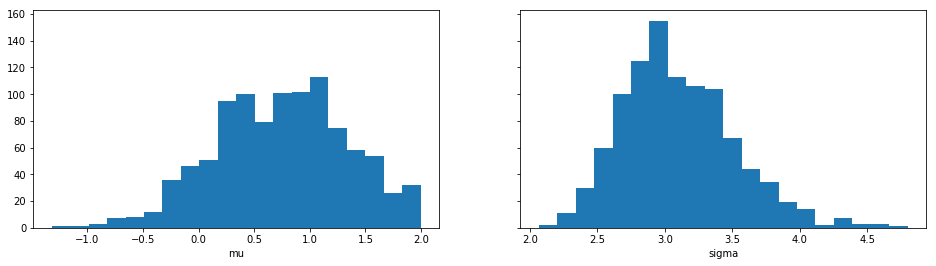
We can try to infer the true generating parameters mean0 and std0 above with any of ELFI’s inference methods. Let’s use ABC Rejection sampling and sample 1000 samples from the approximate posterior using threshold value 0.5:

Method: Rejection
Number of samples: 1000
Number of simulations: 120000
Threshold: 0.492
Sample means: mu: 0.748, sigma: 3.1

Let’s plot also the marginal distributions for the parameters: